This post is meant to discuss the probabilistic clock synchronization technique. The main goal of this technique is to bound the difference between systems by setting up an upper bound. Formally, we define the problem as \(|P(t)-Q(t)|\leq \varepsilon\), or the difference between clocks across the network. We will go over the technical detains and discuss what these symbols represent in later sections. Most of these materials are from Prof. Mok’s slides on dependable systems classes.

Perfect Synchronization

The motivation behind this technique is that synchronization always involves overheads. In a perfect environment where network delay and request processing time are both 0, the clocks can be synchronized with ease. A slave P will send ‘‘Time = ?’’ at global time \(t\) to master Q and master Q replies ‘‘Time = Q(t)’’ instantaneously at global time \(t\). Then P will adjust its clock P(t) according to Q(t). However, such case only exists in imagination.

Amortization

Suppose the difference between the clock of P and Q is \(\Delta\) at synchronization, our goal is to adjust P’s logical clock C(t) to mitigate the difference. The adjustment is simple:

\[C(t)=H(t)+A(t)\]

Here C(t) is P’s logical clock, H(t) is P’s hardware clock, and A(t) is the adjustment function(can also be A(H(t))).

A naive method will be simply subtract or add \(\Delta\) to C(t) to mitigate the difference. However, it will create a discontinuity in P’s clock, which may disrupt systems services. For example, if \(\Delta = 2\) seconds,the logical clock will instantly jump ahead 2 seconds and a stopwatch will skip one second.

So the adjustment function is as follows:

\[A(t)=m\cdot H(t)+N\]

Now the logical clock can be derived as follows:

\[C(t)=(1+m)\cdot H(t)+N\]

This process is called amortization.

However, how do we know the value for m and N? Let’s take a look at the time when amortization process starts, the logical time of P at this moment is:

\[L=(1+m)\cdot H+N \qquad (1)\]

At the end of the amortization (lasts for time period \(\alpha\)) we have reached \(M=H+\alpha\). Here M is the master logical clock sent by master Q. So at the end of the amortization, the slave P should be able to catch up with its master’s logical clock after \(\alpha\) period of time. Therefore, we have:

\[M+\alpha = (1+m)(H+\alpha)+N \qquad (2)\]

Solving (1) and (2) together, we now get:

\[m = \frac{M-L}{\alpha}\]

\[N = L - (1+m)H\]

Thus, at the end of amortization at time \(t\) where \(t > H+\alpha\), we would want the following to be true:

\[C(t)=C(H+\alpha)+(H(t)-H(H+\alpha))=H(t)+M-H\]

Here is a question, why is N required in this case. Couldn’t we simply use m to amortize the time difference? Here’s my interpretation(feel free to pin me if you have something else in mind): if N is set to be 0, then at the beginning of amortization, we would have:

\[L=(1+m)H\]

Therefore, \(m = \frac{L-H}{H}\) . Now, m is settled by L and H. Compared to \(m=\frac{M-L}{\alpha}\) , we can see that now m is a constant and not determined by the value of \(\alpha\). We lost control of the amortization rate \(m\), which is not desirable.

General Case

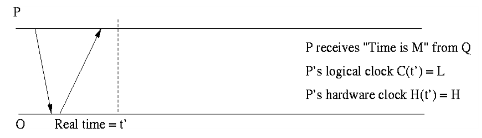
We now return to the general case where network delay and processing time are both present. The situation is represented below:

Looking at this graph, we can see slave P takes 2d real time to for a round-trip. Let’s also assume that 2D is the round-trip delay measured by P’s clock between sending and receiving. Then we can bound the clock time 2D based on the drift rate \(\rho\) of the clock:

\[2d(1-\rho)\leq 2D \leq2d(1+\rho)\]

Ignoring higher order terms of \(\rho\), we now have \(2d\leq(1+\rho)2D\).

When looking at the graph above, one thing to notice is we are not sure of the time \(\alpha\) and \(\beta\). However, if we are going to pick one, \(\beta\) will be more important than \(\alpha\). This is because if we know the value of \(\beta\), then we know the lower bound of the round-trip delay. Here we assume min is the minimum amount of time required for network transfer, \(\beta\) will be the time master Q spends between processing the request and responds the result back to P.

Now we’ve narrowed down our focus to \(min+\beta\). The time interval between \(Q(t)=T\) and the arrival of ‘‘Time=T’’ at P will be at least \(min(1-\rho)\). This is based on \(\beta=0\) and clock drift rate.

The upper bound of the interval will be \((min+\beta)(1+\rho)\), assuming no time is wasted for \(Q\) to wait until it starts processing the request from P. The time required will be \(min+\beta\) and we need to take Q’s drift rate \(\rho\) into account. We can also see that the total round-trip real time is \(2d=2min+\alpha+\beta\). Thus we get:

\[\beta=2d-2min-\alpha \leq 2d-2min\]

With this equation, we can see that the upper bound measured from Q(t)=T is also bounded. Thus, we have:

\[ \begin{eqnarray} (min+\beta)(1+\rho) &\leq& (min+2d-2min)(1+\rho) \nonumber \newline &=& (2d-min)(1+\rho) \nonumber \newline &=&(1+\rho)2d-min(1+\rho) \nonumber \newline &\leq&(1+\rho)2D(1+\rho)-min(1+\rho) \nonumber \newline &=&(1+2\rho +\rho^2)2D-min(1+\rho) \nonumber \newline &\approx&(1+2\rho )2D-min(1+\rho) \nonumber \end{eqnarray} \]

Now we can see that master Q’s clock time when P receives the response is bounded in the interval \([T+min(1-\rho), T+2D(1+2\rho )-min(1+\rho)]\). The take away here is that we can’t use real time t in a distributed system because it’s merely an abstract concept since all systems in a network essentially rely on their own clock time. We need to find the relationship between T and master’s clock cycle because P will rely on T, not real time \(t\).